基于R的多项式回归检验
小可爱们好,我终于找到了篇涉及多项式回归且公开了数据与代码的文章,所以我们今天一起来复现一下吖。
Flynn, F. J., & Lide, C. R. (2022). Communication Miscalibration: The Price Leaders Pay for Not Sharing Enough. Academy of Management Journal. https://doi.org/10.5465/amj.2021.0245
整体介绍
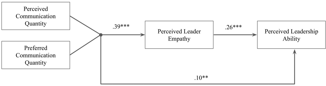
这篇文章想要证明:在对领导沟通错误评估时,领导沟通不足比领导沟通过度更可能形成领导缺乏同情心的感知,进而影响到员工对领导能力的评估。
假设分别为:
- 假设1:管理者可能更常被视为沟通不足而非沟通过度。
- 假设2:当领导者的沟通被认为是良好的,员工会比被误判的时候提供更多有利的评价。
- 假设3a:沟通不足的领导者被认为比沟通过度的领导者具有更少的同理心。
- 假设3b:沟通不足的领导者被认为比沟通过度的领导者具有更低的领导能力。
- 假设4:沟通不足对领导力评价的负面影响将被感知到的缺乏同理心所中介。
各研究分别为:
- 研究1a:使用360评估的档案数据,根据描述人工编码沟通不足与沟通过度,检验假设1;
- 研究1b:招募了400名被试,采用量表衡量与领导的沟通情况(1=沟通不足,5,=沟通良好,9=沟通过度),检验假设1;
- 研究2:招募了350名被试,操纵了领导的沟通情况(3种),采用单因素方差分析检验假设2-4;
- 研究3:采用多项式回归的方式,检验假设1-4。
本次主要分享多项式回归的处理方式,仅以Study 3 为例。
公开数据
获取地址:https://osf.io/fkqhb/?view_only=9415b6468fbf4e8f9041af0dac2c8d43
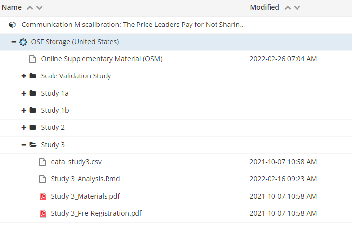
作者非常nice的直接分享了.Rmd文件,我们下载后打开即可。
结果复现
软件准备
安装R包
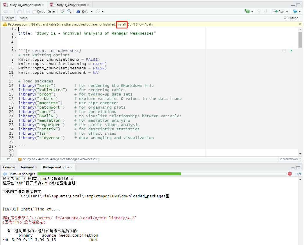
打开.Rmd文件后,Rstudio大概率会提醒你,有未安装的包。我们直接点击【Install】,等待即可。
前期准备
# set knitting options
knitr::opts_chunk$set(echo = FALSE)
knitr::opts_chunk$set(warning = FALSE)
knitr::opts_chunk$set(message = FALSE)
knitr::opts_chunk$set(comment = NA)
这里的意思是设置knitr参数,作用是加强代码的可读性,和数据分析无关。
# load packages
library("knitr")        # for rendering the RMarkdown file
library("kableExtra")   # for rendering tables
library("broom")        # for tyding-up data sets
library("tibble")       # explore variables & values in the data frame
library("magrittr")     # use pipe operator
library("patchwork")    # for organizing plots
library("corrr")        # for correlations
library("GGally")       # to vizualize relationships between variables
library("mediation")    # for mediation analysis
library("emmeans")      # for planned contrasts
library("reghelper")    # for simple slopes analysis
library("lme4")         # for linear mixed effects models
library("lavaan")       # for mediation
library("semPlot")      # for mediation
library("ggpubr")       # for plots
library("car")
library("RSA")
library("Rmisc")        # for error bars on plots
library("rstatix")      # for basic stats tests
library("tidyverse")    # data wrangling and visualization
加载R包。
# set graph themes
source("psych290RcodeV1.R")
这一步我运行时会报错,大概是我没有"psych290RcodeV1.R"这个文件吧。但这也不影响数据分析。
# IMPORT CLEANED DATA
df.data <- read.csv("data_Study3.csv")
作者原始语句是读取"data/data_Study3.csv",但是公开数据中.Rmd和.csv 是在同一个文件夹里,所以我把语句调整了下。
假设1
# paired t-test
t.test(df.data$actual, df.data$ought,
       paired = TRUE)
对数据中的actual和ought列进行配对样本t检验。
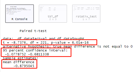
由此可得文中橙色部分数据。
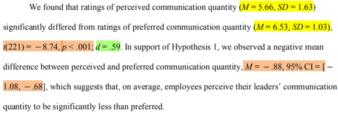
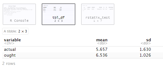
    ## group-level descriptive stats
    df.data %>%
      select(actual, ought) %>%
      get_summary_stats(., type = "mean_sd") %>%
      select(-n)
对actual和ought列进行描述性统计,由此可得黄色部分数据。
# effect size
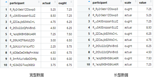
## transform data
df.data_long <- df.data %>%
select(participant, ought, actual) %>%
pivot_longer(., cols = c(ought, actual),
names_to = "scale")
将宽型数据(即一个ID拥有多个变量,此处为222行)转换为长型数据(即一个ID与一个变量为一行,此处形成444行。)
    ## calculate cohen's d
    cohens_d(df.data_long, value ~ scale, paired = TRUE)
计算组间差异效应量cohen’s d,由此可得绿色部分数据。
假设2-一致性更优
数据准备
#-------------------
# DATA PREPARATION
#-------------------
df <- df.data %>%
  select(ability, empathy, X = actual, Y = ought)
选择df.data文件中的【ability, empathy, actual, ought】四列形成一个新的数据文件,名为【df】,其中将actual改命名为X,ought改命名为Y。
# # center predictors at the grand mean
grandmean <- mean(c(df$X, df$Y), na.rm=T)
df$X <- df$X-grandmean
df$Y <- df$Y-grandmean
此处为中心化。语句含义为:计算X与Y的均值,再用原X/Y减去均值,形成新的X/Y。
# add squared and interaction terms of the predictors (required to inspect multicollinearity)
df$X2 <- df$X^2
df$XY <- df$X*df$Y
df$Y2 <- df$Y^2
此处为计算平方项与交互项。
# inspect potential multicollinearity using the variance inflation factor (VIF),
# (see Fox, 2016 for a discussion of VIFs and their cutoffs)
lm_sqd <- lm(ability ~ X + Y + X2 + XY + Y2, data=df)
vif(lm_sqd)
使用方差膨胀因子(VIF)检查潜在的多重共线性。具体的衡量标准,可以去看Fox(2016)。
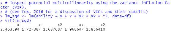
作者这里的结果都没超过3,所以是不存在多重共线性的。
检验假设
#------------------------------------------------------------------------
# TEST THE CONGRUENCE HYPOTHESIS FOR THE OUTCOME VARIABLE ability
#------------------------------------------------------------------------

# ESTIMATE THE POLYNOMIAL MODEL
rsa_sqd <- RSA(ability ~ X*Y, data=df, model="full")
这里就是把我们传统的回归分析(lm或者glm)改成了多项式回归的分析方式(RSA)。
含义依旧是对结果变量【ability】做关于X与Y的多项式回归,数据来自df,model选择“full”,最终将这个分析的结果储存为【rsa_sqd】,方便后续调用。
# GET PARAMETERS
## congruence hypothesis supported if...
### 1) p10 is n.s.
### 2) p11 confidence interval includes 1
### 3) a3 is n.s.
### 4) a4 is significant and negative


getPar(rsa_sqd) %>%
  filter(label %in% c("b0", "b1", "b2", "b3", "b4", "b5",
                      "p10", "p11",
                      "a1", "a2", "a3", "a4")) %>%
  mutate_at(.vars = vars(c(est, se, pvalue, ci.lower, ci.upper)),
            .funs = ~ round(., 4)) %>%
  select(-z)

### *NOTE* - a1 is significant, meaning there is a linear common main effect of X and Y (i.e., the effect of congruence on perceived ability strengthens as employees report greater quantities of actual and expected communication)
这里啥也不用改,直接运行即可。
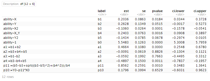
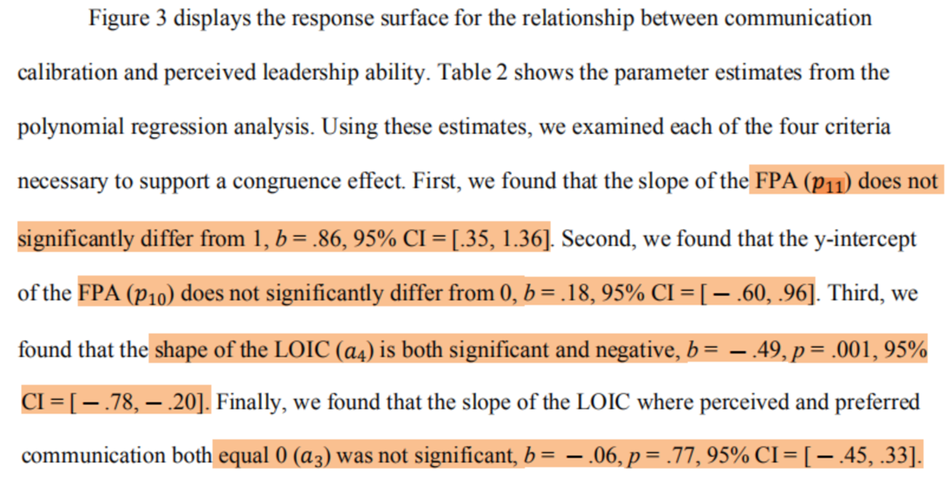
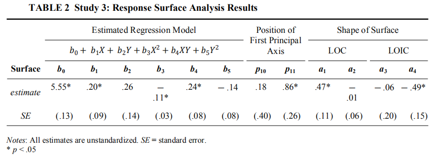
关于一致性假设成立的条件是:①不一致性线(L=-T)上 ,斜率(a3)不显著,曲率(a4)为负且显著;②第一主轴没有偏离一致性线(L=T),即斜率 p 11=1、截距p10=0。所以这里的假设得到了验证。
绘制图形
#------------------------------------------------------------------------
# PLOTS
#------------------------------------------------------------------------
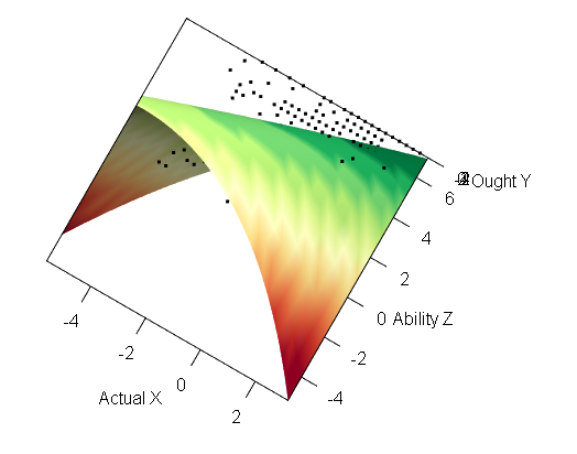
# ESTIMATED MODEL
plot(rsa_sqd, legend=F, param=F,
axes=c("LOC", "LOIC","PA1"),
project=c("LOC", "LOIC","PA1"),
xlab="Perceived\nQuantity", ylab="Preferred\nQuantity", zlab="Perceived Ability")
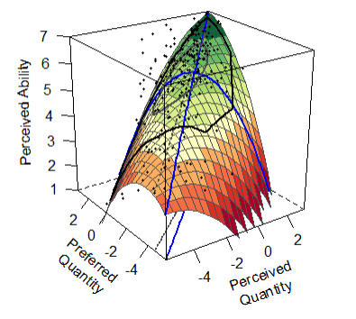
作者文章中的图就是这张。
# CONTOUR MODEL
plot(rsa_sqd, type="contour",
     xlab="Actual X", ylab="Ought Y", zlab="Ability Z")
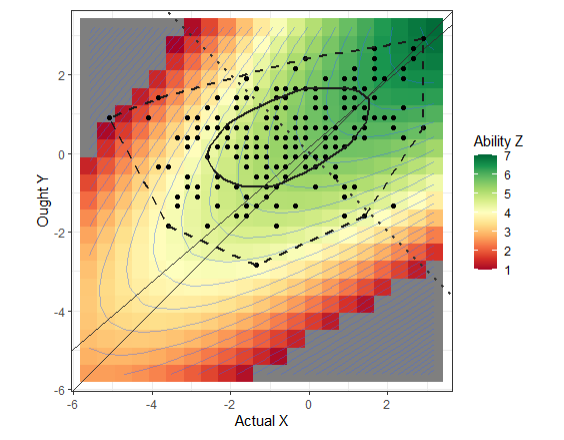
# # INTERACTIVE MODEL
plot(rsa_sqd, type="interactive",
      xlab="Actual X", ylab="Ought Y", zlab="Ability Z")
后面这两张只是不同的作图形式,并非一定要汇报。
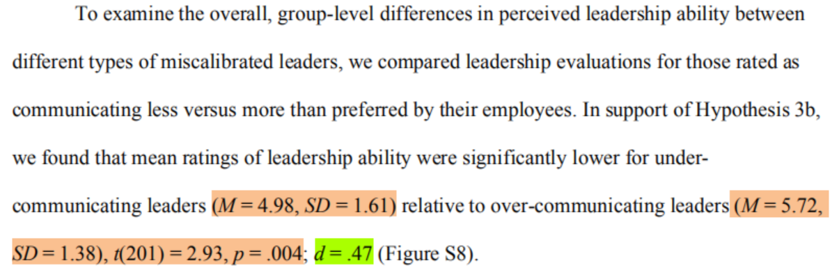
假设3b-不对称性
# t-test
df.data %>%
  filter(communication %in% c("over","under")) %>%
  t.test(ability ~ communication, data = .,
         var.equal = TRUE)

    ## group-level descriptive stats
    df.data %>%
      filter(communication %in% c("over","under")) %>%
      group_by(communication) %>%
      get_summary_stats(ability, type = "mean_sd") %>%
      select(-n)
这里是独立样本t检验,大致上和H1相同,就不展开啦。
# effect size
lsr::cohensD(df.data$ability[df.data$communication == "under"],
       df.data$ability[df.data$communication == "over"])
换了一种方式计算组间差异效应量cohen’s d,结果不再是表,而是一个具体的数字。
# visualization
ability_errorBars <- summarySE(df.data, measurevar = "ability", groupvars = "communication") %>%
  mutate_at(.vars = vars(communication),
            .funs = ~ recode(., `under` = "Under-Communicates",
                             `calibrated` = "Well-Calibrated",
                             `over` = "Over-Communicates")) %>%
  mutate_at(.vars = vars(communication),
            .funs = ~ factor(., levels = c("Under-Communicates", "Well-Calibrated", "Over-Communicates")))

ggplot(data = ability_errorBars,
       mapping = aes(x = communication,
                     y = ability)) +
  geom_bar(position = "dodge", stat = "identity", color = "black", width = .5) +
  geom_errorbar(aes(ymin = ability-se, ymax = ability+se),
                width = .15, position = position_dodge(.5)) +
  theme_Publication_leaveLegend() +
  scale_fill_grey() +
  coord_cartesian(ylim = c(0,8)) +
  scale_y_continuous(limits = c(0,8), expand = c(0,0)) +
  labs(x = "\nLeader Communication Calibration",
       y = "Perceived Ability\n",
       title = "")
# ggsave("Study 3_leader ability_withSE.png", dpi = 800)
可视化的部分,因为我前面没办法加载出"psych290RcodeV1.R",所以会报错。等我搞定再复现它。
假设4-中介效应
# define the block variable function
block.poly = function(y, m, x, z, controls, data, boot.n) {
	require(lavaan)
	# Setup the variables that will be used in the analysis
	data$b_y = data[,y]
	data$b_m = data[,m]
	data$b_x = data[,x]
	data$b_z = data[,z]

	# standardize and create the polynomial components
	data$b_x_std = scale(data$b_x, center=T, scale=T)
	data$b_z_std = scale(data$b_z, center=T, scale=T)
	data$b_x_std_sq = data$b_x_std^2
	data$b_z_std_sq = data$b_z_std^2
	data$b_x_stdXb_z_std = data$b_x_std*data$b_z_std

	# First, create the block variable for the polynomial components predicting the mediator
	frmla = as.formula("b_m ~ b_x_std + b_z_std + b_x_std_sq + b_x_stdXb_z_std + b_z_std_sq")
	bl_1 = lm(frmla, data=data)
	bl_1_co = summary(bl_1)$coefficients[2:6,1]
	bl_1_vars = names(bl_1_co)

	# Second, create the block info predicting the outcome
	frmla = as.formula(paste(y,"~",paste0(controls, collapse="+"),"+b_x_std + b_z_std + b_x_std_sq + b_x_stdXb_z_std + b_z_std_sq", sep=""))
	bl_2 = lm(frmla, data=data)
	bl_2_co = summary(bl_2)$coefficients[(length(controls)+2):(length(controls)+6),1]
	bl_2_vars = names(bl_2_co)

	data$bl_1_var = 0
	data$bl_2_var = 0
	for(i in 1:5) {
		data$bl_1_var = data$bl_1_var + bl_1_co[i]*data[,bl_1_vars[i]]
		data$bl_2_var = data$bl_2_var + bl_2_co[i]*data[,bl_2_vars[i]]
	}

	line1 = paste("b_m ~ ",paste0(controls, collapse="+"), "+ b1*bl_1_var", sep="")
	line2 = paste("b_y ~ ",paste0(controls, collapse="+"), "+ bl_2_var + b2*b_m", sep="")
	line3 = "a1 := b1*b2"
	path.model = paste(line1, line2, line3, sep="\n")
	o = sem(model=path.model, data=data, se="boot", bootstrap=boot.n)
	return(o)
}

# the defined parameter a1 is the indirect effect of the congruence variables (perceived and preferred communication quantity) on the ultimate outcome (perceived ability) through the mediator (perceived empathy)
这个部分就是固定的,相当于设置一个固定程序,我们在使用时只需要定义好x、m、y、z以及对应的数据文件即可。
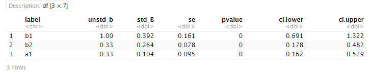
# 5000 bootstrapped samples (no controls)
out = block.poly(y="ability",m="empathy",x="actual",z="ought", controls=NULL,
                 data=df.data, boot.n=5000)
parameterestimates(out, standardized = TRUE) %>%
  filter(label %in% c("b1", "b2", "a1")) %>%
  select(label, unstd_b = est, std_B = std.all, se, pvalue, ci.lower, ci.upper)
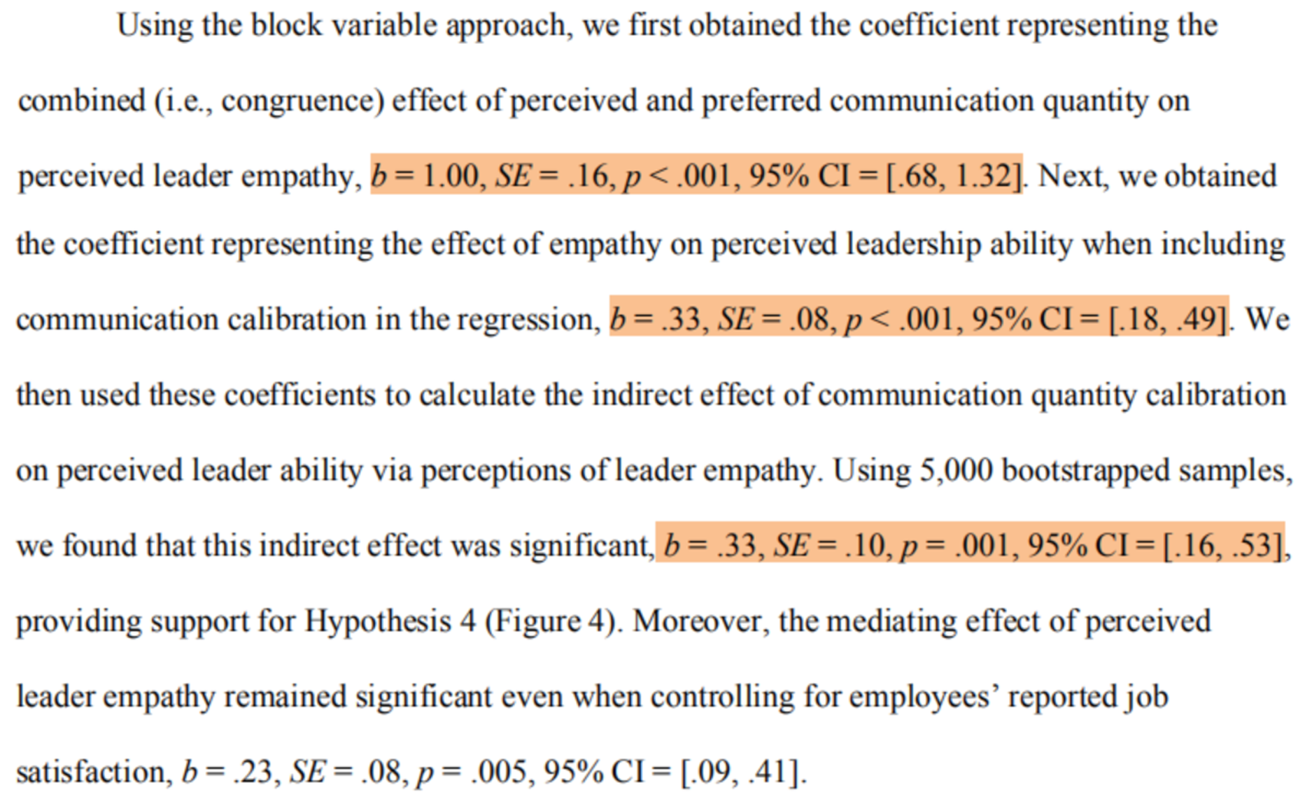
# 5000 bootstrapped samples (controlling for job satisfaction)
out_controlJS = block.poly(y="ability",m="empathy",x="actual",z="ought", controls="job_satisfaction",data=df.data, boot.n=5000)
parameterestimates(out_controlJS, standardized = TRUE) %>%
  filter(label %in% c("b1", "b2", "a1")) %>%
  select(label, unstd_b = est, std_B = std.all, se, pvalue, ci.lower, ci.upper)
如果有控制变量,就在controls=" “中加入即可。
其他
作者在最后提供了描述性统计和信度等信息,我们这里受限于篇幅,也就不展开啦,有兴趣的小可爱可以自己尝试哦。
啦啦啦,这篇推送就到这里了。它比我预期耗时久多了,所以又拖到了现在TAT。
但是实操一遍后,萜妹还是很有收获的。强烈推荐对多项式回归感兴趣的小可爱们试试。
参考文献:
Fox, J. (2016). Applied Regression Analysis and Generalized Linear Models, 3e. Thousand Oaks, CA: Sage Publications
下期预告:《范文丨顶刊引言精读(十)》
往期推送:
原文链接: